On June 16, 2019, an industrial engineering portal published Balanceo de Líneas, where Dr. Eliyahu Goldratt is quoted as saying "An hour lost in the bottleneck is an hour lost in the whole system", but the article lacked analyzing the lines as systems.
The conclusion of that article is that balancing manufacturing or assembly lines reduces unit costs, and further says that “The balance or line balancing it is one of the most important tools for production management, since a balanced manufacturing line depends on the optimization of certain variables that affect the productivity of a process, (…) "
In this article I will start the exposition precisely from the phrase of Dr. Goldratt, who did various experiments to show that balancing the capacities in a line reduces the productivity of the system, increasing the cost of production.
Manufacturing or assembly lines as systems
A system is a set of interdependent elements with a purpose. A manufacturing or assembly line conforms to this definition: each workstation is dependent on another and together they have the purpose of creating a product from raw material.
One of the main characteristics of a system is that it requires the synchronization of all the parts for the result to be produced. In this sense, the production of a product is an emergent result of the system as a whole. None of the parts is capable of producing it by itself, not even a subset of them. This is easy to demonstrate. If the above were true, that subset is our system and the rest is left over.
In this sense, we need all parties to generate the product. This was obvious, however what is not so obvious is understanding how we achieve maximum productivity from a system.
In reality there is variability
To make the demonstration required to refute the aforementioned article, I will begin by establishing a fact of reality. The processing time of a unit on a workstation is a time within a range, it is not a specific number of minutes.
For example, when in a station we say that a product takes 2 minutes, we know that that is an average, but that it could be 1 minute or 5 minutes.
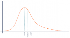
Regarding the process times, we know that they have a marked asymmetry to the right. See the following graphic:

By making our process time measurements on a workstation, considering the process of identical parts, after a large number of cases we obtain a table of results with a large dispersion.
It could never be processed in 0 seconds or less, which was obvious. In a few cases the process was achieved in 50-70 seconds, most of the cases are between 70 and 120 seconds, but not a few cases are in the range between 120 and 250 seconds. Actually, we see that half of the cases are in the last range.
In my experience of more than fifteen years, this graph represents the reality of the vast majority of processes in all types of factories.
Although I know that there is a difference between the median and the mean (or average), I will use the average for simplicity. And we can say that a process has a 50% probability of being running at its average or faster. This I will use next in the next demo.
Effect of process dependency
Variability affects all resources. We are going to distinguish the variability due to common causes from that which has special causes. Special causes are all those that are easily identifiable, for example, a power outage.
Common causes are many and varied, and for all practical purposes, the causes that stop one process do not necessarily affect other processes. Therefore, the productivity of one process in one instant may be above its average while that of another is below it.
Let us now consider a generic line (manufacturing or assembly):
We have a flow direction and we know that a resource cannot process anything if it has not received material from the previous one.
Let's design our process to produce 10 units per hour. After a while, the process is up and running and all resources are processing what they can.
Let's see what happens if we balance the line, that is, all resources have an average capacity of 10 u / h (or an average time of 6 minutes per unit).
We already know that the probability of producing 10 u / h or more is 50%. Let's look at what happens in the first two resources in the first three hours:
|
Periods |
Resource 1 |
Recurso 2 |
Total production |
|
First hour |
7 u/h |
15 u/h |
7 u/h |
|
Second hour |
14 u/h |
6 u/h |
6 u/h |
|
Third hour |
9 u/h |
9 u/h |
9 u/h |
Despite the fact that on average each one of the resources is capable of making 10 u / h, when combining them in each period, as the capacities are not synchronized, what Dr. Goldratt said is fulfilled: the system moves at the rhythm of the slowest.
Didn't we already know this? Sure you do, but capacity balancing, which is one of the techniques taught in many college courses, ignores the systemic effect of the combination.
By extending this effect to the rest of the resources, we can easily see that the probability that a balanced line will produce at the average design speed is approximately 0.5n, where n is the number of resources chained on the line. In this case, with 7 resources, the probability of achieving 10 u / h of finished product is ~ 0.8%, that is, in a year of 300 work days, only 2 would reach the design productivity of the line.
The better the balance, the worse the performance.
What happens to the cost when balancing the lines?
From the above conclusion, we now know that we will have ~ 20% fewer finished products compared to the original plan (or worse), so all the production cost associated with operating the line (discounted raw material) will be divided into less products, which will increase the real unit cost by 25% (or more).
So, to reduce the total unit cost (the only one that is relevant) it is necessary to ensure that the system maximizes its productivity as a whole, and not the productivity of each of the resources.
What if it is an assembly line?
Normally one sees factories where resources are isolated from each other and material (WIP for work in progress) has to be moved from one center to another. But with the idea of speeding up the process, and following the model attributed to Ford, some lines are arranged in a way where there is no room to accumulate WIP and the entire line advances at the same time.
Now that you know what happens when balancing a line, take a look at what happens with an assembly line, even if it is not balanced!
Unable to accumulate WIP between resources, the entire line advances at the slowest pace. But which one is the slowest? Let's look at the graph again:
Towards the right side we have "the tail" of the distribution, and we have already seen that it is not at all improbable that a resource is in that productive cycle.
Unlike the general case, where the little WIP that can be accumulated does allow some resources to cushion somewhat the effect of dependency, in the case of the assembly line this is not possible. In this case, the entire line moves at the rate of the resource that is operating in its tail.
If one has 7 resources coupled, we already know that the probability that at least one is in the tail is 99%. If the line has a few dozen stations (such as assemblers for bulky products such as automobiles), it is certain that they are operating well below their averages.
On an assembly line it becomes incredibly relevant to reduce variability, leading the company to a flood of improvement projects that cost a lot of time and money. And it is not possible to eliminate the tails of the distributions either. It seems like a sisífea task to improve productivity.
Even Elon Musk regrets so much automation in the line of Tesla, although I am not sure if he already noticed the effect that I just described or has other reasons, but he sees that his results are below what was planned.
The solution is to find the resource that is the constraint of the entire system (has the smallest average capacity) and isolate it, allowing WIP to accumulate before and after. This will raise the overall productivity of the system quite a bit. And yes, I realize the investment that is required to modify the layout, but with an increase of only 10% in total productivity, I am sure that this project is profitable.
"If we don't balance the line, there is a lot of waste"
In our example, suppose that the third resource is our constraint, the one with an average capacity of 10 u / h, and the rest have 20 u / h or more.
First I clarify that the double is not an exaggeration. The capacity of the line to recover when there are losses, or in other words, to absorb the variability, depends on this extra capacity. If the excess over the restriction is small, we still have a problem with variability. In my experience, this extra capacity, which in Theory of Constraints (TOC) jargon is called protective capacity, must exceed 30-50% and sometimes more.
So we see that if we feed the line with all the material that the first one is capable of processing, in a short time we have an intolerable accumulation of WIP in the corridors of the plant, because the constraint is not capable of draining that WIP. In fact, what happens is that one has the sensation that the bottleneck is moving inside the plant. The latter is one of the symptoms of the opposite, that there is excess capacity. And when there is excess WIP, there are several effects by which capacity is wasted, even in the constraint. And here the phrase "an hour lost in the bottleneck, is an hour lost in the whole system" applies.
We must control the amount of WIP to ensure that the constraint always has work but that it is not so much that it wastes capacity. In another article I will delve into how capacity is wasted with excess WIP.
This WIP control mechanism must release material to process at the rate dictated by the constraint, so all other resources will have idle times. But these idle times are not real wastes of capacity; they are actually waiting times for the system to synchronize to the rhythm of the constraint. In TOC jargon this is a buffer, which is the mechanism for achieving maximum productivity.
That is why I have written that, many times, LEAN implementations, understood as waste reduction, are the enemy of productivity.
In addition, an operator receives the same salary if he operates a machine of greater or lesser capacity. So the salary expense does not change if one has more capacity machines. Look at the prices of the machines and you will see that doubling the capacity does not cost twice the investment.
All the times that are generated like this are not waste, and are excellent for practicing 5S or for doing preventive maintenance.
Now may be a good time to reformulate the productivity measurement. If production orders are what is needed and no more, when “idle” time increases, it is a sign that productivity has increased.
"I don't know, something doesn't add up ..."
To demonstrate the effect of line balancing, I suggest an experiment that you can do at home or with your work team.
Get 100 tokens and 7 dice, and build a production line with 7 stations. Each station is assigned a die, which will be our variability simulation. Note that the die is not asymmetric, because it is uniform between 1 and 6, although it may exaggerate the spread. But it is a good simulator of variable capacity.
If the simulation of a workday is done, each station rolls its die and produces at most the number it rolled. If you roll a 5 and have three chips, you can only pass to the next 3 chips. The tokens that are going to be passed to me in the same turn cannot be used. The first resource "produces" what the die rolled because it has an unlimited supply of tokens.
What is the average capacity of a die? It is the average of all your numbers. The sum is 1 + 2 + 3… + 6 = 21 and that divided by six gives 3.5. So each station has an average capacity of 3.5 units / day. In 20 days they should be able to make 70 units.
To start the experiment on steady state, distribute 4 chips to each one, and now do 20 days of production.
Compare what you got to the expected 70 units.
This experiment saves hours of discussion and mathematical proofs, and is much more fun. Then variations can be made to demonstrate other things, such as that moving people from one place to another only increases the variability but does not get more capacity.
Conclusion
Balancing the production line only reduces the total capacity of the line. Worse still, the actual capacity is considerably less than planned, so it will default on a large proportion of the orders, in addition to the obvious effect on invoiced sales.
Al Autor,
creo que hay un gran error en la premisa inicial, lo que describes no es un línea productiva, estas describiendo una máquina, ya que todas las operaciones son secuenciales (sin pulmones entre etapas), y sólo en ese caso la probabilidad total es el producto de las probabilidades parciales.
Hay otro error en tu análisis, cuando diseñas una línea de producción, te preocupas que la mayor inversión sea tu limitante de capacidad total, y que todas las otras operaciones tengan un costo de inversión menor y que tengan flexibilidad para mantener el pulmón del recurso principal alimentado.
Tu análisis sólo se puede aplicar a máquinas, como una línea productiva de autos, que funciona como tal, una máquina.
Hola Alberto
Primero lo último: la línea sin pulmones la describí al final, es la que llamé línea de montaje y es donde cité a Elon Musk.
Respecto de tu descripción de cómo diseñar una línea de producción, es una perfecta explicación de NO balancear capacidades: estoy de acuerdo.
En el ejercicio descrito sí se permite tener pulmones, y no hace mucha diferencia. no me apoyé en esa premisa para la conclusión. En todo caso, en este sitio cualquiera puede salir de dudas para convencerse de que balancear líneas perjudica la productividad del sistema: https://www.the-dice-game.com/
¡Muchas gracias por leer y comentar!
Impecable Matías!
Gracias Víctor.